Model Optimization is a module of Tencent Cloud TI-ONE Platform (TI-ONE) for inference acceleration. This module uses TI Acceleration Service (TI-ACC) capabilities to optimize the inference acceleration of the models in Model Repository, while reducing costs and improving efficiency. It is currently free for a limited time, but the models optimized through this module can only be used for inference services in Model Services of TI-ONE.
Optimization Task List
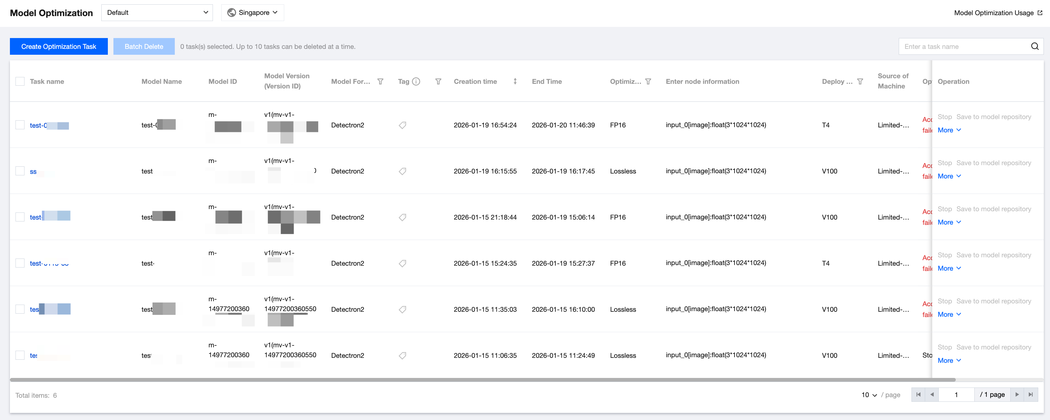
The optimization task list allows you to view information such as the optimization task name, optimization progress, and acceleration ratio, and perform operations such as saving optimized models to Model Repository. The optimization progress provides statuses like Starting, Accelerating, and Acceleration Completed, and the optimization process usually takes several minutes to complete.
You can click Stop to stop an optimization task in progress (Starting or Accelerating) immediately.
You can save the task in the Acceleration Completed status for service release. You can click Save to Model Repository to immediately save the model optimized through this optimization task to the model optimization list page of Model Repository.
You can re-accelerate the task that fails during acceleration. You can choose More > Re-accelerate to edit and accelerate the optimization task again.
You can click Delete to delete an optimization task immediately.
You can click Edit Tag to edit a tag.
Creating an Optimization Task
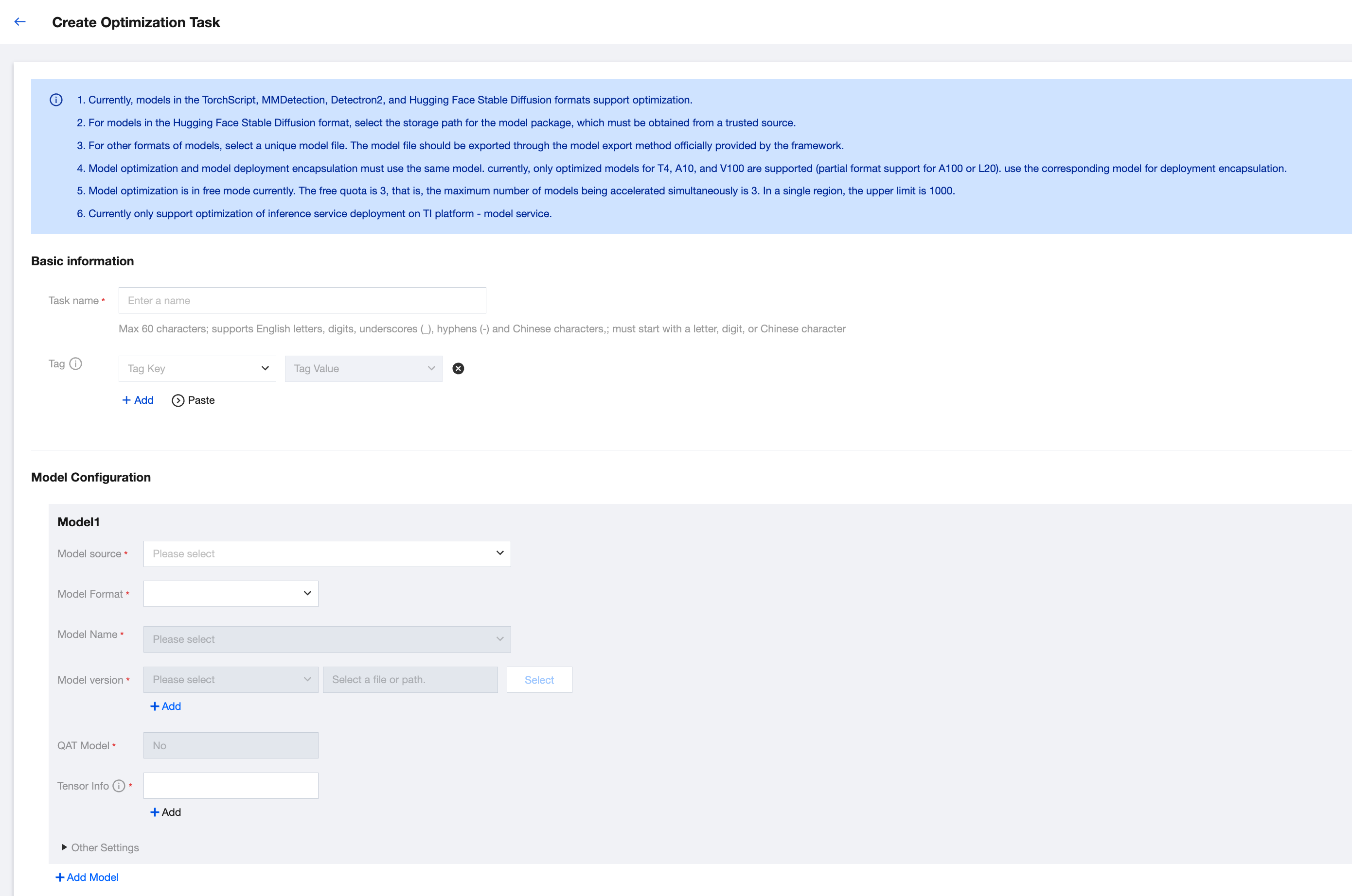
Currently, models in TorchScript, MMDetection, Detectron2, Hugging Face-Stable Diffusion, ONNX, Savedmodel, and Frozen Graph formats are supported. You can refer to the following guidance for integration.
1. Enter a task name. When only a model and its version are optimized, the task name should be the one you entered. When multiple models or versions are added, multiple optimization tasks will be generated, and the name of each task consists of the task name you entered + -model name + -model version + # + a sequence number.
2. Add a tag as needed.
3. Select a model source. The selected model source should be consistent with the model source field in Model Repository. The model name will be filtered based on the selected model source.
4. Select a model name, which refers to the name of the model to be optimized. You can add multiple models and versions for an optimization task. When multiple models or versions are added, multiple optimization tasks will be generated, and the name of each task consists of the task name you entered + -model name + -model version + # + a sequence number.
5. Select a model version, which refers to the version of the model to be optimized. You can select multiple versions and their corresponding files.
6. Select a model file, which refers to the specific file of the model to be optimized. Model files in different formats have different suffixes. For details, see the specific prompts.
7. Quantization-Aware Training (QAT) is a technique used in deep learning to train models that can be quantized and allow these models to be deployed on the hardware with limited computation capabilities. QAT simulates quantization during training and allows modules to adapt to lower bit-widths while maintaining accuracy. Unlike Post-Training Quantization (PTQ) which quantizes pre-trained models, QAT involves quantizing models during training.
Note:
The QAT process can be broken down into the following steps:
1. Define a model: Define a floating-point model, which is identical to a general model.
2. Define a quantized model: Define a quantized model that has the same structure as the original model but includes quantization operations (such as torch.quantization.QuantStubQ) and dequantization operations (such as torch.quantization.DeQuantstub()).
3. Prepare the data: Prepare the training data and quantize it to the appropriate bit-width.
4. Train a model: During training, use the quantized model for forward and backward passes, and calculate the accuracy loss using dequantization operations when each epoch or batch ends.
5. Perform quantization again: During training, quantize the model parameters again using dequantization operations and continue training using new quantization parameters.
6. Fine-tuning: Use the fine-tuning technology to further improve the model accuracy after the training is completed.
8. Fill in the Tensor Information field:
Input data should be considered as a whole. The shape information of input data must be provided in advance before model optimization, to ensure that the model optimization task is performed normally.
Input data uses multidimensional tensors as its basic elements, consisting of lists (list), dictionaries (dict), tuples (tuple), and their nested combinations.
For each element in the input data, you need to provide its shape size. The shape size of each element can be represented in the element:dtype(shape) format, and each element occupies one line.
element is represented as follows:
For Layer 1 of the input data:
If this layer is a list or tuple, each element is represented as input_0, input_1, ...; particularly, if the input data is a single tensor, it is represented as input_0.
If this layer is a dict, each element is represented as the key of the dict.
For Layer n (n > 1) of the input data:
If this layer is a list, each element is represented as [0], [1], ...
If this layer is a tuple, each element is represented as (0), (1), ...
If this layer is a dict, each element is represented as [key].
dtype is the basic data type of an element, for example, float, int32, and array.char.
shape is the actual shape of an element. There are 3 cases:
Fixed size: represented by a size value. size consists of n positive integers separated by asterisks (*). For example, 3*1024*1024 indicates that the element is a 3-dimensional tensor with a size of 3 x 1024 x 1024.
Dynamic and continuous size: represented by 2 size values separated by a comma (,). For example, 3*1024*2048,3*2048*2048 indicates that the element is a variable-sized 3-dimensional tensor, with a minimum size of 3 x 1024 x 2048 and a maximum size of 3 x 2048 x 2048.
Dynamic and discrete size: represented by a list of size values. For example, [3*1024*1024,3*2048*2048] indicates that the element is a variable-sized 3-dimensional tensor, with 2 possible sizes: either 3 x 1024 x 1024 or 3 x 2048 x 2048.
Example configurations:
Example 1: The input data is a single tensor.
The tensor has a fixed size, its data type is float, and its actual shape size is 1 x 3 x 1024 x 1024.
The Tensor Information field is filled in with 1 line, namely, input_0:float(1*3*1024*1024).
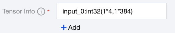
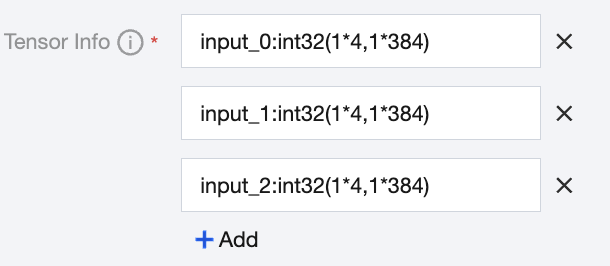
Example 2: The input data is a single-layer list.
There are 3 elements, all of which are tensors with the data type int32, and their actual shape sizes are dynamic and continuous sizes with a minimum value of 1 x 4 and a maximum value of 1 x 384.
The Tensor Information is filled in with 3 lines, namely, with input_0:int32(1*4,1*384), input_1:int32(1*4,1*384), and input_2:int32(1*4,1*384).
Example 3: The input data is a single-layer dict.
There are 3 elements, their keys are input_ids, input_mask, and segment_ids respectively, their values are all tensors with the data type int32, and their actual shape sizes are dynamic and continuous sizes with a minimum value of 1 x 128 and a maximum value of 8 x 128.
The Tensor Information is filled in with 3 lines, namely, input_ids:int32(1*128,8*128), input_mask:int32(1*128,8*128), and segment_ids:int32(1*128,8*128).
9. The latest acceleration library engine version is used by default, and the latest acceleration library engine version varies for each format.
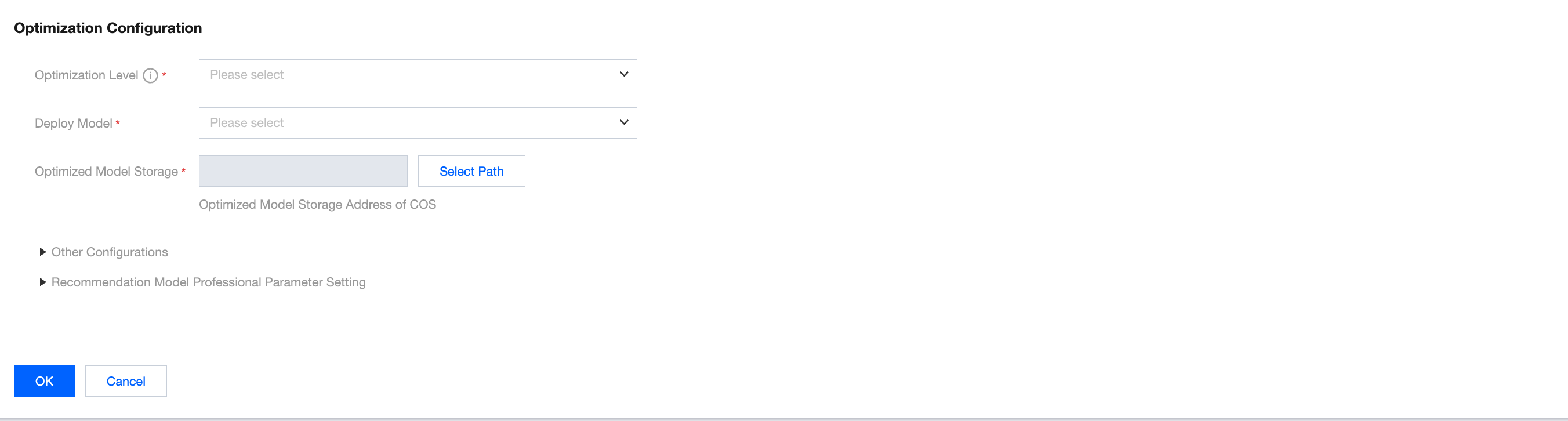
10. Optimization Level can be FP16 or Lossless. Lossless indicates that the optimization is performed based on the original model accuracy, while FP16 indicates that the optimization is performed based on the FP16 accuracy. It is recommended to use FP16 to perform the optimization because it offers faster inference than the lossless method and generally does not cause accuracy degradation.
11. The deployment instance type can be T4, V100, or A10, and A100 or PNV5b is supported only for certain model formats. When PNV5b is selected, Resource Group is required. When T4 is used, you can select Time-Limited Free (Pay-as-You-Go) or Resource Group. If you select other instance types, only the free mode is supported. The deployment instance type selected during optimization must be consistent with the instance type of the actual deployment service. That is, if a T4 deployment service is needed, the instance type should be set to T4 here.
12. You can click Select Path to select the location for storing the optimized model. This path cannot overlap with the main directory of the original model. When you click Save to Model Repository for a model in the Acceleration Completed status, all files in the original model directory will be copied to a newly generated m-xxx/mv-xxx folder under this path, and the optimized model tiacc.pt will be generated and stored in the model folder. If you want to deploy the optimized model, Model Package Specifications of TI-ONE must be followed.
13. After you click OK, the optimization task is performed, and the optimization task list page is displayed.
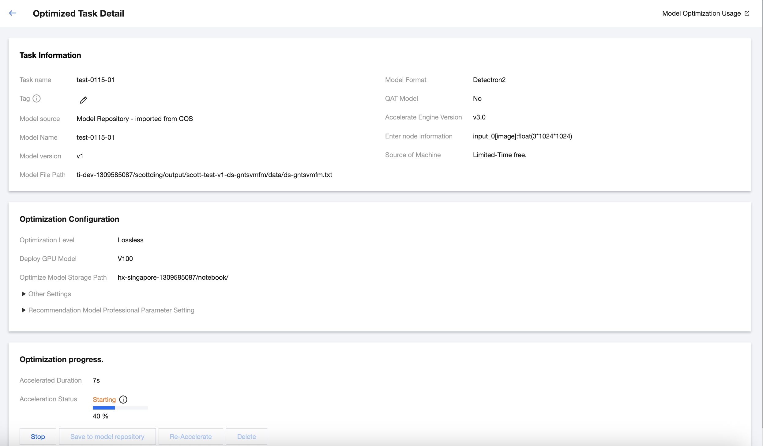
Optimized Task Details
You can click the optimized task name to go to the optimization task details page. On this page, you can view the detailed task information and optimization report, and perform corresponding operations.